Gaussian Processes

The main concept of Gaussian process is, as the name suggests its a process(anything that deals with time) that has basically an infinate dimensional gaussian distribution associated with it.

1. Gaussian Distribution
- 1.1 Why Gaussian?
- 1.2 Multivariate Gaussian
2. Stochastic Process
3. GP INIT
4. GP KERNEL
5. Why Gaussian Process?
References

1. Gaussian Distribution

Gaussian

\[Y \sim N(0,1)\] \[PDF: f_Y(y) = \frac{1}{\sigma\sqrt{2\pi}} \exp\left( -\frac{1}{2}\left(\frac{y-\mu}{\sigma}\right)^{\!2}\,\right)\]

1.1 Why Gaussian?

Family of normal/gaussian distribution is closed under linear operations
TODO: Write proof for above. (Addition, Multiplication, Convolution, Integration, Diffrentation of gaussians.)
Central Limit Theorem
Sum/mean of large random variables will converge to gaussian.
Max Entropy
Infinitely divisible
If jointly normal & uncorrelated, then they are independent
Square-loss functions lead to procedures that have a gaussian probabilistic interpretation

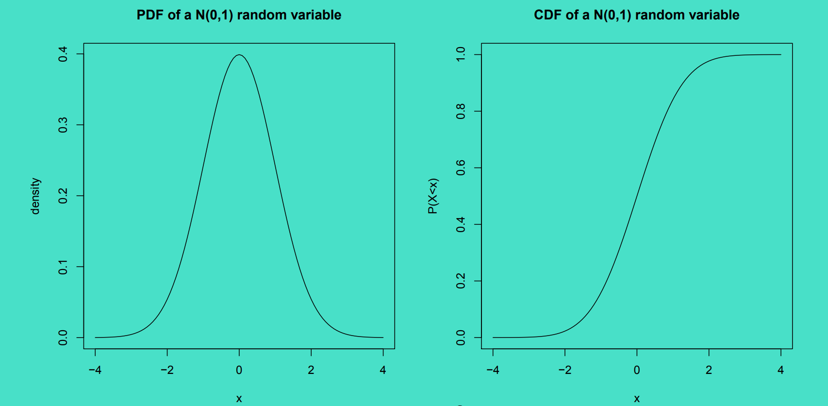
1.2 Multivariate Gaussian

Mean Vector: $\mu \in R^d$
covariance matrix: $\Sigma \in R^{d \times d}$
For bivariate case: d = 2, $y = \begin{pmatrix}y1 \\ y2 \end{pmatrix}, \ \mu = \begin{pmatrix} \mu1 \\ \mu2 \end{pmatrix}$, $\Sigma = \begin{pmatrix}\sigma_1^2 & \rho \sigma_1 \sigma_2 \\ \rho \sigma_1 \sigma_2 & \sigma_2^2\end{pmatrix}$

TODO: Attach the screenshot and link of the interactive to understand multivatiate covariances.(Temp attached) 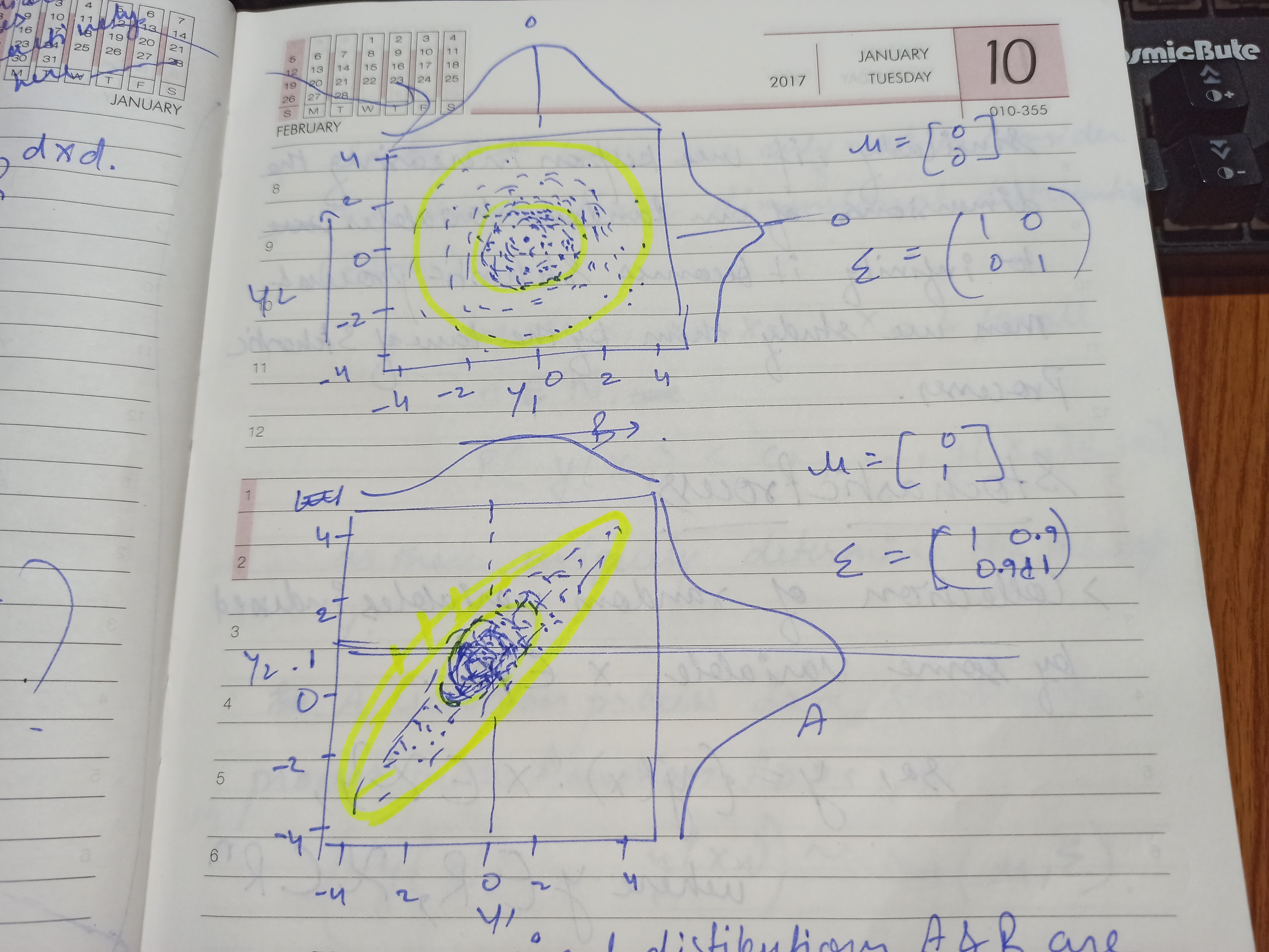Gaussian

In the second plot from above figure, it shows marginal distributions A and B are still same, look exactly similar. Just the correlation factor is being changed.
Higher the correlation, knowing one variable $y1$ is essentially equivalent to $y2$ , basically precision increases.

Similarly, if we keep on increasing the dimension of our random variables to infinity it becomes Stochastic Process and then we study them by the law of Stochastic Processes.

2. Stochastic Process

Collection of random variables indexed by some variable $x \in \chi$
so, $y = \{y(x):x \in \chi \},$ where $y \in R, \chi \subset R^n$.

Now, as we use Daniell-Kolmogorov theorem(Stchostic and measure theory) for stochastic processes so by that law we only need to consider the finite dimensional ditribution(FDDs), i.e. for all $x_1, x_2, x_3, ..... x_n$ and for all n $\in N, P(y(x_1) \leq c_1, ... , y(x_n) \leq cn )$ as these uniquely determine the law of y.

A Gaussian Process is a stochastic process with Gaussian FDD, i.e. $(y(x_i), ... , y(x_n)) \sim N_n(\mu, \Sigma)$ .

In other words,
$y(\cdot) \sim GP(m(\cdot), k(\cdot,\cdot))$
where $E(y(x)) = m(x)$
$$Cov(y(x), y(x’) = k(x,om variables will converge to gaussian.

x’)$<br> and$x $&$ x’$$ are basically the indexes/location for dimension.

3. GP INIT

We can choose any mean and covariance, but generally the most popular choice is $m(x) = 0$ .
K must be positive semi-definate function inorder to have our covarivance matrix in valid form for computation .
Stationary Process: We often assume $k$ is a function of only the distance between locations. $Cov(y(x), y(x'))= k(x-x')$ .
If $Cov(y(x), y(x'))= k(\Vert x-x' \Vert)$ , then the covariance function is said to be isotropic.
$k$ determines the hypothesis space or space of functions.

4. GP KERNEL

GP’s inherit its properties from the covariance function k. Mainly Smoothness, Differentiability and Variance. Here are the most widely used kernels:

4.1 RBF Kernel: Radial Basis Function Kernel.

Curves generated by RBF Kernel are infinitely differentiable i.e. derivaties of all order,hence they are analytic functions.
\[k(x,x') = \exp\left(-\frac{1}{2} \frac{(x- x')^{2}}{l}\right)\]

4.2 Matern 3/2 Kernel:

\[k(x,x') =(1 + |x-x'|) \exp(-|x-x'|)\]
only 1 time differentiable.
$matern \ 5/2$ is 2 time differentiable,$matern \ 7/2$ is 3 times, and so on. So for $matern \ \infty/2$,it gets converged to RBF Kernel.

4.3 Brownian Motion Kernel:

\[k(x,x') = min(x,x')\]
No where differentiable, very rough function.

4.4 White Noise Kernel:

\[k(x,x')= \left\{ \begin{array}{ll} 1 & \mbox{if $x=x'$}\\ 0 &\mbox{otherwise} \end{array} \right\}\]
Basically they can be thought of as a derivative of Brownian Motion.

TODO: Attach the screenshot and link of the interactive for various GP kernels.

5. Why Gaussian Process?

Closed under addition.
Closed under Bayesian conditioning, i.e. if we observe $D = (F(x_1), F(x_2), F(x_3),...., F(x))$ , then $F | D \sim$ GP with updated mean and covariance functions.
Closed under any linear operation. If $f \sim GP(m(\cdot), k(\cdot,\cdot))$ , then if $\mathcal{L}$ is a linear operator.

continued…….

Cited as:

@article{kartik2021gp,
  title   = "Gaussian Processes",
  author  = "Paliwal, Kartik",
  journal = "kartikpaliwal.ml",
  year    = "2021",
  url     = "https://kartikpaliwal.ml/posts/Gaussian-Processes/"
}

References

[1] Hyun Oh Song et al. “Deep Metric Learning via Lifted Structured Feature Embedding.” CVPR 2016. [code]